Robust effect sizes for 2 independent groups

When I was an undergrad, I was told that beyond a certain sample size (n=30 if I recall correctly), t-tests and ANOVAs are fine. This was a lie. I wished I had been taught robust methods and that t-tests and ANOVAs on means are only a few options among many alternatives. Indeed, t-tests and ANOVAs on means are not robust to outliers, skewness, heavy-tails, and for independent groups, differences in skewness, variance (heteroscedasticity) and combinations of these factors (Wilcox & Keselman, 2003; Wilcox, 2012). The main consequence is a lack of statistical power. For this reason, it is often advised to report a measure of effect size to determine, for instance, if a non-significant effect (based on some arbitrary p value threshold) could be due to lack of power, or reflect a genuine lack of effect. The rationale is that an effect could be associated with a sufficiently large effect size but yet fail to trigger the arbitrary p value threshold. However, this advise is pointless, because classic measures of effect size, such as Cohen’s d, its variants, and its extensions to ANOVA are not robust.

To illustrate the problem, first, let’s consider a simple situation in which we compare 2 independent groups of 20 observations, each sampled from a normal distribution with mean = 0 and standard deviation = 1. We then add a constant of progressively larger value to one of the samples, to progressively shift it away from the other. As illustrated in Figure 1, as the difference between the two groups increases, so does Cohen’s d. The Matlab code to reproduce all the examples is available here, along with a list of matching R functions from Rand Wilcox’s toolbox.

Figure 1. Examples of Cohen’s d as a function of group differences. For simplicity, I report the absolute value of Cohen’s d, here and in subsequent figures.

We can map the relationship between group mean differences and d systematically, by running a simulation in which we repeatedly generate two random samples and progressively shift one away from the other by a small amount. We get a nice linear relationship (Figure 2).

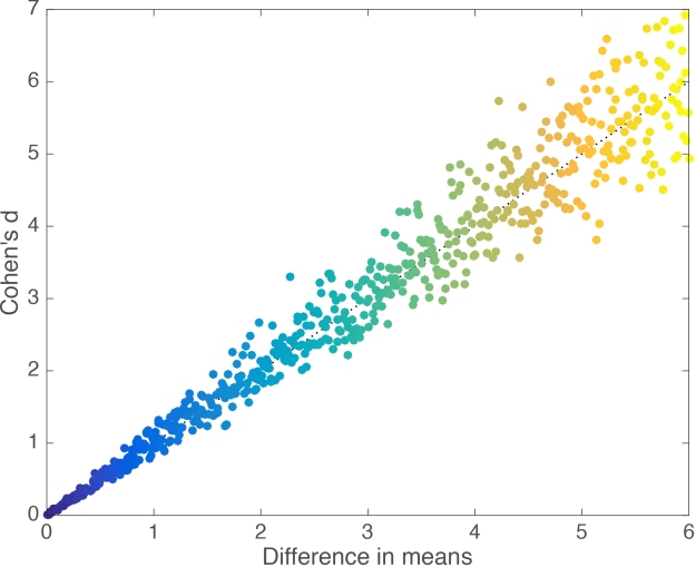
Figure 2. Linear relationship between Cohen’s d and group mean differences.

Cohen’s d appears to behave nicely, so what’s the problem? Let’s consider another example, in which we generate 2 samples of 20 observations from a normal distribution, and shift their means by a fixed amount of 2. Then, we replace the largest observation from group 2 by progressively larger values. As we do so, the difference between the means of group 1 and group 2 increases, but Cohen’s d decreases (Figure 3).

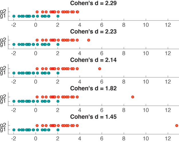
Figure 3. Cohen’s d is not robust to outliers.

Figure 4 provides a more systematic illustration of the effect of extreme values on Cohen’s d for the case of 2 groups of 20 observations. As the group difference increases, Cohen’s d wrongly suggests progressively lower effect sizes.

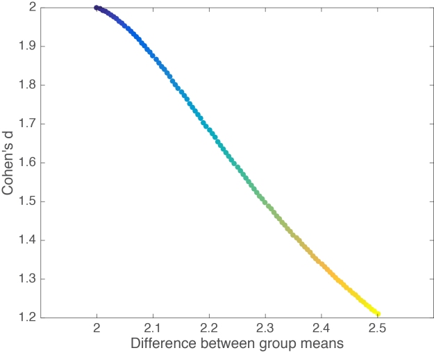
Figure 4. Cohen’s d as a function of group mean differences in the presence of one outlier. There is an inverse and slightly non-linear relationship between the two variables.

What is going on? Remember that Cohen’s d is the difference between the two group means divided by the pooled standard deviation. As such, neither the numerator nor the denominator are robust, so that even one unusual value can potentially significantly alter d and lead to the wrong conclusions about  effect size. In the example provided in Figure 4, d gets smaller as the mean difference increases because the denominator of d is composed of a non-robust estimator of dispersion, the variance, such that the outlier increases variability, which leads to an increase of the denominator, and thus a lower d. The outlier also has a strong effect on the mean, which leads to an increase of the numerator, and thus larger d. However, the outlier has a stronger effect on the variance than the mean: this imbalance explains the overall decrease of d with increasing outlier size. I leave it as an exercise to understand the origin of the non-linearity in Figure 4. It has to do with the differential effect of the outlier on the mean and the variance.

One could argue that the outlier value added to one of the groups could be removed, which would solve the problem. There are 3 objections to this argument:

• there are situations in which extreme values are not outliers but expected and plausible observations from a skewed or heavy tail distribution, and thus physiologically or psychologically meaningful values. In other words, what looks like an outlier in a sample of 20 observations could well look very natural in a sample of 200 observations;
• for small sample sizes, relatively small outliers could go unnoticed but still affect effect size estimation;
• outliers are not the only problem: skewness & heavy tails can affect the mean and the variance and thus d.

For instance, in some cases, two groups can differ in skewness, as illustrated in Figure 5. In the left panel, the two kernel density estimates illustrate two samples of 100 observations from a normal distribution. The two groups overlap only moderately, and Cohen’s d is high. In the right panel, group 1, with a mean of zero, is the same as in the previous panel; group 2, with a mean of 2, is almost identical to the one in the left panel, except that its largest 10% observations were replaced with slightly larger observations. As a result, the overlap between the two distributions is the same in the two panels – yet Cohen’s d is quite smaller in the second example.

Figure 5. Cohen’s d for normal & skewed distributions.

The point of this example is to illustrate the potential for discrepancies between a visual inspection of two distributions and Cohen’s d. Clearly, in Figure 5, a useful measure of effect size should provide the same estimates for the two examples. Fortunately, several robust alternatives have this desirable property, including Cliff’s delta, the Kolmogorov-Smirnov test statistic, Wilcox & Muska’s Q, and mutual information.

Robust versions of Cohen’s d

Before going over the 4 robust alternatives listed above, it is useful to consider that Cohen’s d is part of a large family of estimators of effect size, which can be described as the ratio of a difference between two measures of central tendency (CT), over some measure of variability:

(CT1 – CT2) / variability

From this expression, it follows that robust effect size estimators can be derived by plugging in robust estimators of central tendency in the numerator and robust estimators of variability in the denominator. Several examples of such robust alternatives are available, for instance using trimmed means and Winsorised variances (Keselman et al. 2008; Wilcox 2012). R users might want to check these functions from Wilcox for instance:

• akp.effect
• yuenv2
• med.effect

There are also extensions of these quantities to the comparison of more than one group (Wilcox 2012).

Robust & intuitive measures of effect sizes

In many situations, the robust effect sizes presented above can bring a great improvement over Cohen’s d and its derivatives. However, they provide only a limited perspective on the data. First, I don’t find this family of effect sizes the easiest to interpret: having to think of effects in standard deviation (or robust equivalent) units is not the most intuitive. Second, this type of effect sizes does not always answer the questions we’re most interested in (Cliff, 1996; Wilcox, 2006).

The simplest measure of effect size: the difference

Fortunately, effect sizes don’t have to be expressed as the ratio difference / variability. The simplest effect size is simply a difference. For instance, when reporting that group A differs from group B, typically people report the mean for each group. It is also very useful to report the difference, without normalisation, but with a confidence or credible interval around it, or some other estimate of uncertainty. This simple measure of effect size can be very informative, particularly if you care about the units. It is also trivial to make it robust by using robust estimators, such as the median when dealing with reaction times and other skewed distributions.

Probabilistic effect size and the Wilcoxon-Mann-Whitney U statistic

For two independent groups, asking by how much the central tendencies of the two groups differ is useful, but this certainly does not exhaust all the potential differences between the two groups. Another perspective relates to a probabilistic description: for instance, given two groups of observations, what is the probability that one random observation from group 1 is larger than a random observation from group 2? Given two independent variables X and Y, this probability can be defined as P(X > Y). Such probability gives a very useful indication of the amount of overlap between the two groups, in a way that is not limited to and dependent on measures of central tendency. More generally, we could consider these 3 probabilities:

• P(X > Y)
• P(X = Y)
• P(X < Y)

These probabilities are worth reporting in conjunction with illustrations of the group distributions. Also, there is a direct relationship between these probabilities and the Wilcoxon-Mann-Whitney U statistic (Birnbaum, 1956; Wilcox 2006). Given sample sizes Nx and Ny:

U / NxNy = P(X > Y) + 0.5 x P(X = Y)

In the case of two strictly continuous distributions, for which ties do not occur:

U / NxNy = P(X > Y)

Cliff’s delta

Cliff suggested to use P(X > Y) and P(X < Y) to compute a new measure of effect size. He defined what is now called Cliff’s delta as:

delta = P(X > Y) – P(X < Y)

Cliff’s delta estimates the probability that a randomly selected observation from one group is larger than a randomly selected observation from another group, minus the reverse probability (Cliff, 1996). It is estimated as:

delta = (sum(x > y) – sum(x < y)) / NxNy

In this equation, each observation from one group is compared to each observation in the other group, and we count how many times the observations from one group are higher or lower than in the other group. The difference between these two counts is then divided by the total number of observations, the product of their sample sizes NxNy. This statistic ranges from 1 when all values from one group are higher than the values from the other group, to -1 when the reverse is true. Completely overlapping distributions have a Cliff’s delta of 0. Because delta is a statistic based on ordinal properties of the data, it is unaffected by rank preserving data transformations. Its non-parametric nature reduces the impact of extreme values or distribution shape. For instance, Cliff’s delta is not affected by the outlier or the difference in skewness in the examples from Figure 3 & 5.

For an MEEG application, we’ve used Cliff’s delta to quantify effect sizes in single-trial ERP distributions (Bieniek et al. 2015). We also used Q, presented later on in this post, but it behaved so similarly to delta that it does not feature in the paper.

An estimate of the standard error of delta can be used to compute a confidence interval for delta. When conditions differ, the statistical test associated with delta can be more  powerful than the Wilcoxon-Mann-Whitney test, which uses the wrong standard error (Cliff, 1996; Wilcox, 2006). Also, contrary to U, delta is a direct measure of effect size, with an intuitive interpretation. There are also some attempts at extending delta to handle more than two groups (e.g. Wilcox, 2011). Finally, Joachim Goedhart has provided an Excel macro to compute Cliff’s delta.

Update: Cliff’s delta is also related to the later introduced “common-language effect size” – see this post from Jan Vanhove.

All pairwise differences

Cliff’s delta is a robust and informative measure of effect size. Because it relies on probabilities, it normalises effect sizes onto a common scale useful for comparisons across experiments. However, the normalisation gets rid of the original units. So, what if the units matter? A complementary perspective to that provided by delta can be gained by considering all the pairwise differences between individual observations from the two groups (Figure 6). Such distribution can be used to answer a very useful question: given that we randomly select one observation from each group, what is the typical difference we can expect? This can be obtained by computing for instance the  median of the pairwise differences. An illustration of the full distribution provides a lot more information: we can see how far away the bulk of the distribution is from zero, get a sense of how large differences can be in the tails…

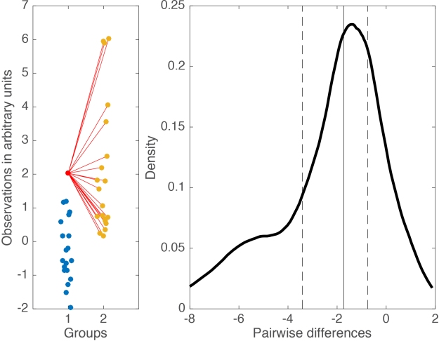
Figure 6. Illustration of all pairwise differences. Left panel: scatterplots of the two groups of observations. One observation from group 1 (in red) is compared to all the observations from group 2 (in orange). The difference between all the pairs of observations is saved and the same process is applied to all the observations from group 1. Right panel: kernel density estimate of the distribution of all the pairwise differences between the two groups. The median of these differences is indicated by the continuous vertical line; the 1st & 3rd quartiles are indicated by the dashed vertical lines.

Something like Figure 6, in conjunction with Cliff’s delta and associated probabilities, would provide a very useful summary of the data.

When Cohen’s d & Cliff’s delta fail

Although robust alternatives to Cohen’s d considered so far, including Cliff’s delta, can handle well situations in which 2 conditions differ in central tendency, they fail completely to describe situations like the one in Figure 7. In this example, the two distributions are dramatically different from each other, yet Cohen’s d is exactly zero, and Cliff’s delta is very close to zero.

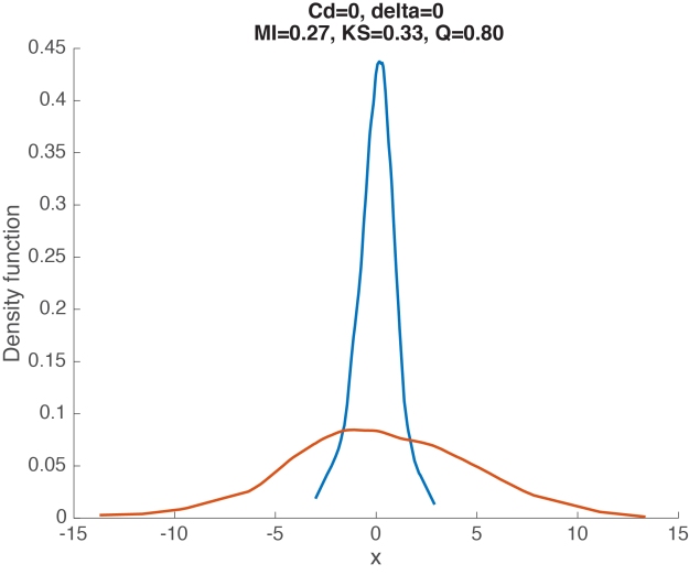
Figure 7. Measures of effect size for two distributions that differ in spread, not in location. Cd = Cohen’s d, delta = Cliff’s delta, MI = mutual information, KS = Kolmogorov-Smirnov test statistics, Q = Wilcox & Muska’s Q.

Here the two distributions differ in spread, not in central tendency, so it would wise to estimate spread instead. This is indeed one possibility. But it would also be nice to have an estimator of effect size that can handle special cases like this one as well. Three estimators fit the bill, as suggested by the title of Figure 7.

The Kolmogorov-Smirnov statistic

It’s time to introduce a powerful all-rounder: the Kolmogorov-Smirnov test statistic. The KS test is often mentioned to compare one distribution to a normal distribution. It can also be used to compare two independent samples. In that context, the KS test statistic is defined as the maximum of the absolute differences between the empirical cumulative distribution functions (ecdf) of the two groups. As such KS is not limited to differences in central tendency; it is also robust, independent of the shape of distributions, and provides a measure of effect size bounded between 0 and 1. Figure 8 illustrates the statistic using the example from Figure 7. The KS statistic is quite large, suggesting correctly that the two distributions differ. More generally, because it is robust and sensitive to differences located anywhere in the distributions, the KS test is a solid candidate for a default test for two independent samples. However, the KS test is more sensitive to differences in the middle of the distributions than in the tails. To correct this problem, there is also a weighted version of the KS test which provides increased sensitivity to differences in the tails of the distributions – check out the ks R function from Wilcox.

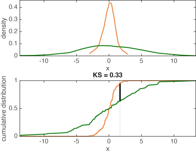
Figure 8. Illustration of the KS statistic for two independent samples. The top panel shows the kernel density estimates for the two groups. The lower panel shows the matching empirical cumulative distribution functions. The thick black line marks the maximum absolute difference between the two ecdfs – the KS statistic. Figure 8 is the output of the ksstat_fig Matlab function written for this post.

The KS statistic non-linearly increases as the difference in variance between two samples of 100 observations progressively increases (Figure 9). The two samples were drawn from a standard normal distribution and do not differ in mean.

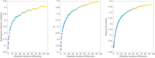
Figure 9. Relationship between effect sizes and variance differences. The 3 measures of effect size illustrated here are sensitive to distribution differences other than central tendency, and are therefore better able to handle a variety of cases compared to traditional effect size estimates.

Wilcox & Muska’s Q

Similarly to KS, the Q statistic is also a non-parametric measure of effect size. It ranges from 0 to 1, with chance level at 0.5. It is the probability of correctly deciding whether a randomly selected observation from one of two groups belongs to the first group, based on the kernel density estimates of the two groups (Wilcox & Muska, 1999). Essentially, it reflects the degree of separation between two groups. Again, similarly to KS, in situations in which two distributions differ in other aspects than central tendency, Q might suggest that a difference exists, whereas other methods such as Cohen’s d or Cliff’s delta would not (Figure 9).

Mutual information

In addition to the KS statistic and Q, a third estimator can be used to quantify many sorts of differences between two or more independent samples: mutual information (MI). MI is a non-parametric measure of association between distributions. As shown in Figure 9, it is sensitive to group differences in spread. MI is expressed in bits and is quite popular in neuroscience – much more so than in psychology. MI is a powerful and much more versatile quantity than any of the tools we have considered so far. To learn more about MI, check out Robin Ince’s tutorial with Matlab & Python code and examples, with special applications to brain imaging. There is also a clear illustration of MI calculation using bins in Figure S3 of Schyns et al. 2010.

In the lab, we use MI to quantify the relationship between stimulus variability and behaviour or brain activity (e.g. Rousselet et al. 2014). This is done using single-trial distributions in every participant. Then, at the group level, we compare distributions of MI between conditions or groups of participants. We thus use MI as a robust measure of within-participant effect size, applicable to many situations. This quantity can then be illustrated and tested across participants. This strategy is particularly fruitful to compare brain activity between groups of participants, such as younger and older participants. Cliff’s delta for instance could then be used to quantify the MI difference between groups.

Comparisons of effect sizes

We’ve covered several useful robust measures of effect size, with different properties. So, which one should be used? In statistics, the answer to this sort of questions often is “it depends”. Indeed, it depends on your needs and on the sort of data you’re dealing with. It also depends on which measure makes more sense to you. The code provided with this post will let you explore the different options using simulated data or your own data. For now, we can get a sense of the behaviour of delta, MI, KS and Q for relatively large samples of observations from a normal distribution. In Figure 10, two distributions are progressively shifted from each other.

Figure 10. Examples of effect size estimates for different distribution shifts.

Figure 11 provides a more systematic mapping of the relationship between effect size estimates and the difference between the means of two groups of 100 observations. The KS statistic and Q appear to have similar profiles, with a linear rise for small differences, before progressively reaching a plateau. In contrast, Cliff’s delta appears to be less variable and to reach a maximum earlier than KS and Q. MI differs from the other 3 quantities with its non-linear rise for small mean differences.

Figure 11. Relationship between effect sizes and mean differences.

To more clearly contrast the 4 effect sizes, all their pairwise comparisons are provided in Figure 12. From these comparisons, it seems that KS and Q are almost completely linearly related. If this is the case, then there isn’t much advantage in using Q given that it is much slower to compute than KS. Other comparisons reveal different non-linearities between estimators. These differences would certainly be worth exploring in particular experimental contexts… But enough for this post.

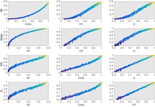
Figure 12. Relationship between effect sizes.

Final notes

Given that Cohen’s d and related estimators of effect size are not robust suggests that they should be abandoned in favour of robust methods. This is not to say that Cohen’s d is of no value – for instance in the case of single-trial ERP distributions of 100s of trials, it would be appropriate (Bieniek et al. 2015). But for typical group level analyses, I see no reason to use non-robust methods such as Cohen’s d. And defending the use of Cohen’s d and related measures for the sake of continuity in the literature, so that readers can compare them across studies is completely misguided: non-robust measures cannot be compared because the same value can be obtained for different amounts of overlap between distributions. For this reason, I am highly suspicious of any attempt to perform meta-analysis or to quantify effect sizes in the literature using published values, without access to the raw data. To allow true comparisons across studies, there is only one necessary and sufficient step: to share your data.

In the literature, there is a rampant misconception assuming that statistical tests and measures of effect size are different  entities. The Kolmogorov-Smirnov test and Cliff’s delta demonstrate that both aspects can be combined elegantly. Other useful measures of effect size, such as mutual information, can be used to test hypotheses by combining them with a bootstrap or permutation approach.

Which technique to use in which situation is something best worked out by yourself, given your own data and extensive tests. Essentially, you want to find measures that are informative and intuitive to use, and that you can trust in the long run. The alternatives described in this post are not the only ones on the market, but they are robust, informative, intuitive, and they cover a lot of useful situations. For instance, if the fields of neuroscience and psychology were to use the Kolmogorov-Smirnov test as default test when comparing two independent groups, I would expect a substantial reduction in the number of false negatives reported in the literature. The Kolmogorov-Smirnov test statistic is also a useful measure of effect size on its own. But because the KS test does not tell us how two distributions differ, it requires the very beneficial addition of detailed illustrations to understand how two groups differ.  This comment applies to all the techniques described in this post, which, although useful, do not provide a full picture of the effects. Notably, they do not tell us how two distributions differ. But detailed illustrations can be combined with robust estimation to compare 2 entire distributions.

References

Bieniek, M.M., Bennett, P.J., Sekuler, A.B. & Rousselet, G.A. (2015) A robust and representative lower bound on object processing speed in humans. The European journal of neuroscience.

Birnbaum ZW. 1955. On a use of the Mann-Whitney statistic

Cliff N. 1996. Ordinal methods for behavioral data analysis. Mahwah, N.J.: Erlbaum

Keselman HJ, Algina J, Lix LM, Wilcox RR, Deering KN. 2008. A generally robust approach for testing hypotheses and setting confidence intervals for effect sizes. Psychol Methods 13: 110-29

Rousselet, G.A., Ince, R.A., van Rijsbergen, N.J. & Schyns, P.G. (2014) Eye coding mechanisms in early human face event-related potentials. J Vis, 14, 7.

Wilcox RR. 2006. Graphical methods for assessing effect size: Some alternatives to Cohen’s d. Journal of Experimental Education 74: 353-67

Wilcox, R.R. (2011) Inferences about a Probabilistic Measure of Effect Size When Dealing with More Than Two Groups. Journal of Data Science, 9, 471-486.

Wilcox RR. 2012. Introduction to robust estimation and hypothesis testing. Amsterdam ; Boston: Academic Press

Wilcox RR, Keselman HJ. 2003. Modern Robust Data Analysis Methods: Measures of Central Tendency. Psychological Methods 8: 254-74

Wilcox RR, Muska J. 2010. Measuring effect size: A non-parametric analogue of omega(2). The British journal of mathematical and statistical psychology 52: 93-110